Network Architectures

Normalization Layers

Todo

Add descriptions of QK Norm

Let X be a tensor of shape [B, C, ...]. All normalization layers do something like the following:

Y = (X - X.mean(dim=...)) / (X.var(dim=..., unbiased=False).sqrt() + eps)   # normalization
Y = Y * weight + bias   # affine transform

The key difference between different normalization layers are:

Across what reduction dimensions are mean are variance computed.
Whether running mean and running variance are tracked (if tracked, train and eval behaviors may differ).
On what dimensions are affine parameters applied.

A simple comparison of common normalization layers is shown below.

Type	BatchNorm	InstanceNorm	LayerNorm
Reduction	batch + spatial	spatial	last \(D\) dims (usually channel + spatial)
Tracked mean/var	yes by default	no by default	not available
Affine	per-channel	per-channel	per-element on the last \(D\) dims

Batch Normalization

torch.nn.BatchNorm1d, torch.nn.BatchNorm2d and torch.nn.BatchNorm3d computes mean and biased variance across all dims except the channel dimension. As a simple example, below are two equivalent forward passes for BatchNorm.

BatchNorm equivalent implementation

import torch
torch.manual_seed(43)
B, C, H, W = 2, 3, 2, 2
x = torch.randn(B, C, H, W)

# pytorch native BN
bn = torch.nn.BatchNorm2d(C, affine=False)
y1 = bn(x)

# custom BN
eps = 1e-5
mean = x.mean(dim=[0,2,3], keepdim=True)
var = x.var(dim=[0,2,3], unbiased=False, keepdim=True)
y2 = (x - mean) / torch.sqrt(var + eps)

print((y1 - y2).norm())

BatchNormXd also contains tracked statistics (running_mean and running_var), which are updated using a moving average weighted by momentum during training, and are used instead of batch statistics in eval mode.

running_mean and running_var

import torch
torch.manual_seed(43)
B, C, H, W = 2, 3, 2, 2

# pytorch native BN
bn = torch.nn.BatchNorm2d(C, affine=False)

# run through some examples to initialize batch stats
sequence_to_init_stats = [torch.randn(B, C, H, W) for _ in range(3)]
for z in sequence_to_init_stats: _ = bn(z)
print(bn.running_mean, bn.running_var)

# compare
x = torch.randn(B, C, H, W)

# compare in eval mode
# in eval mode, bn uses running_mean, running_var
def custom_batch_norm_2d_evalmode(input, running_mean, running_var, eps):
    mean = running_mean[..., None, None]
    var = var[..., None, None]
    out = (input - mean) / torch.sqrt(var + eps)
    return out

bn.eval()
y1 = bn(x)
y2 = custom_batch_norm_2d_evalmode(x, bn.running_mean, bn.running_var, 1e-5)
print((y1 - y2).norm())

# compare in train mode
# in train mode, bn uses batch_mean and batch_var
def custom_batch_norm_2d_trainmode(input, eps):
    mean = input.mean(dim=[0,2,3], keepdim=True)
    var = input.var(dim=[0,2,3], unbiased=False, keepdim=True)
    out = (input - mean) / torch.sqrt(var + eps)
    return out

bn.train()
y1 = bn(x)
y2 = custom_batch_norm_2d_trainmode(x, 1e-5)
print((y1 - y2).norm())

BatchNormXd allows optimizable affine parameters (weight: [C] and bias: [C]) when you set affine=True. They are applied to the channel dimension of the output through elementwise multiplication and addition.

affine parameters

import torch
torch.manual_seed(43)
x = torch.randn(B, C, H, W)

# pytorch native BN
bn = torch.nn.BatchNorm2d(C, affine=True)   # actually affine=True is default
with torch.no_grad():
    bn.weight[:] = torch.randn_like(bn.weight)
    bn.bias[:] = torch.randn_like(bn.bias)
y1 = bn(x)

# custom BN
eps = 1e-5
mean = x.mean(dim=[0,2,3], keepdim=True)
var = x.var(dim=[0,2,3], unbiased=False, keepdim=True)
y2 = (x - mean) / torch.sqrt(var + eps)
y2 = y2 * bn.weight[..., None, None] + bn.bias[..., None, None]

print((y1 - y2).norm())

Instance Normalization

Instance normalization is basically the same as batch normalization, except:

it does not compute mean and variance across the batch dimension;
track_running_stats=False by default, because instance mean/variance does not reflect dataset statistics so it doesn’t make sense to track them.

InstanceNorm equivalent implementation

import torch
torch.manual_seed(43)
x = torch.randn(2,3,2,2)

# pytorch native IN
instnorm = torch.nn.InstanceNorm2d(3, affine=True, track_running_stats=True)   # actually affine=True is default
y1 = instnorm(x)

# custom IN
eps = 1e-5
mean = x.mean(dim=[2,3], keepdim=True)
var = x.var(dim=[2,3], unbiased=False, keepdim=True)
y2 = (x - mean) / torch.sqrt(var + eps)

print((y1 - y2).norm())

Layer Normalization

LayerNorm computes mean and variance over the last \(D\) dimensions (can be specified by use) of an input, which usually include spatial and channel dimensions. The affine parameters are defined for each individual element for the last \(D\) dimensions. Moreover, LayerNorm does not use running mean and variance.

LayerNorm equivalent implementation

import torch
torch.manual_seed(43)
B, C, H, W = 2, 3, 2, 2
x = torch.randn(B, C, H, W)

# pytorch native LN
# you need to specify the shape of the last D dimensions
# LayerNorm will compute mean and variance over these dimensions
# and also define elementwise affine parameters
layernorm = torch.nn.LayerNorm([C, H, W])
with torch.no_grad():
    layernorm.weight[:] = torch.randn_like(layernorm.weight)    # shape [C, H, W]
    layernorm.bias[:] = torch.randn_like(layernorm.bias)        # shape [C, H, W]
y1 = layernorm(x)

# custom IN
eps = 1e-5
mean = x.mean(dim=[1,2,3], keepdim=True)
var = x.var(dim=[1,2,3], unbiased=False, keepdim=True)
y2 = (x - mean) / torch.sqrt(var + eps)
y2 = y2 * layernorm.weight + layernorm.bias

print((y1 - y2).norm())

Transformer Architecture

Self-Attention

Below is a common self-attention architecture, consisting of a few components:

Input linear projection to QKV features
QK norm and positional encoding
Multihead self-attention
Output linear projection

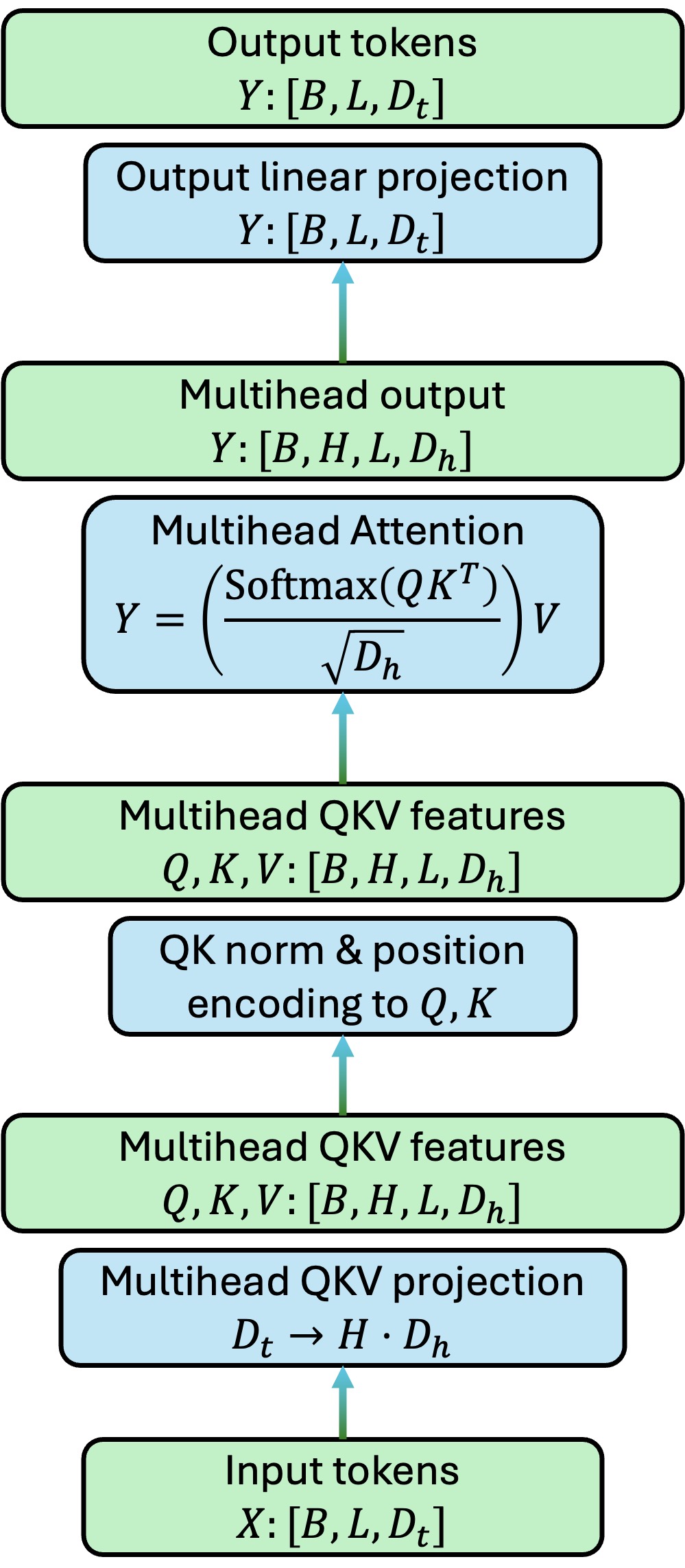
Here \(B\) denotes batch size, \(L\) denotes sequence length (number of tokens) and \(D_t\) denotes token dimensions. Tokens are usually projected to low-dimensional (\(D_h\)-dimensional) multihead (\(H\) heads) QKV features of shape \([B, H, L, D_h]\).

Note

A common practice is to chose \(D_t\) divisible by \(H\) and then set \(D_h=D_t/H\).
In scaling the softmax scores, the head dimension \(D_h\) is used.

A custom implementation of self-attention.

class SelfAttention(torch.nn.Module):
    def __init__(self,
                token_dim: int,
                num_heads: int,
                ):
        super().__init__()
        assert token_dim % num_heads == 0
        head_dim = token_dim // num_heads

        self.token_dim = token_dim
        self.num_heads = num_heads
        self.head_dim = head_dim
        self.qkv_proj = torch.nn.Linear(token_dim, 3 * token_dim)
        self.out_proj = torch.nn.Linear(token_dim, token_dim)
        self.q_norm = torch.nn.LayerNorm(head_dim)
        self.k_norm = torch.nn.LayerNorm(head_dim)

    def forward(self, x: torch.Tensor):
        """
        x: [B, L, Dt]
        """
        B, L, Dt = x.shape
        H, Dh = self.num_heads, self.head_dim
        qkv = self.qkv_proj(x).reshape(B, L, 3, H, Dh)  # [B, L, 3, H, Dh]
        qkv = qkv.permute(2, 0, 3, 1, 4)                # [3, B, H, L, Dh]
        q, k, v = torch.unbind(qkv, dim=0)              # [B, H, L, Dh]

        q = self.q_norm(q)
        k = self.k_norm(k)

        # this part below is usually replaced by scaled_dot_product_attention
        attn_weights = torch.einsum('bhld,bhmd->bhlm', q, k)  # [B, H, L, L]
        attn_weights = attn_weights.softmax(dim=-1)           # [B, H, L, L]
        attn_scale = 1 / math.sqrt(self.head_dim)
        attn_weights = attn_weights * attn_scale              # [B, H, L, L]
        attn_output = torch.einsum('bhlm,bhmd->bhld', attn_weights, v)  # [B, H, L, Dh]
        attn_output = attn_output.permute(0, 2, 1, 3).reshape(B, L, Dt) # [B, L, Dt]

        final_output = self.out_proj(attn_output)
        return final_output

B = 3
L = 5
token_dim = 1024
num_heads = 16

self_attention = SelfAttention(token_dim, num_heads).cuda()
x = torch.randn(B, L, token_dim).cuda()

out = self_attention(x)

Positional Embeddings

In this section we consider positional embedding (PE) for tokens. Suppose we have:

a batch of tokens T: [..., N, D] and

their positions I: [..., N, C].

Usually, I holds the indices for the tokens. For example, if the tokens are structured as a sequence, then C == 1 and I[..., i] == [i]. Or, if the tokens are image patches, then we could have N == H*W, C == 2 and I[..., i*W+j] == [i, j]. This naturally extends to indices of higher dimensions.

Applying PE can usually be formulated as injecting the positional information from I to T, i.e., T_new = apply_PE(T, I), where T_new is also [..., N, D]. It is desired that when tokens in T_new interact with each other, their interaction is affected by the corresponding PE. A common approach is to first obtain a PE code I_new = PE(I) of shape [..., N, D], and then add/multiply I_new to T to get T_new.

Pseudo-code for PE.

def indice_to_PE(I) -> I_new:
    """
    I: [..., N, C], C-dimensional indices of the tokens

    I_new: [..., N, D], embedded indices
    """
    ...

def apply_PE(T, I) -> T_new
    """
    T: [..., N, D], tokens
    I: [..., N, C], C-dimensional indices of the tokens

    T_new: [..., N, D], tokens with PE information
    """
    I_new = indices_to_PE(I)    # [..., N, D]
    T_new = apply_PE(T, I_new)  # [..., N, D]

Sinusoidal Positional Embedding